This is the second part of the GANs episodes, if you missed the first you can check that out here. In the first part, I talked about the why of GANs and a couple of other things, do check it out.
In this part we will be looking at what it takes to build a very simple GAN architecture. Link to Code here.
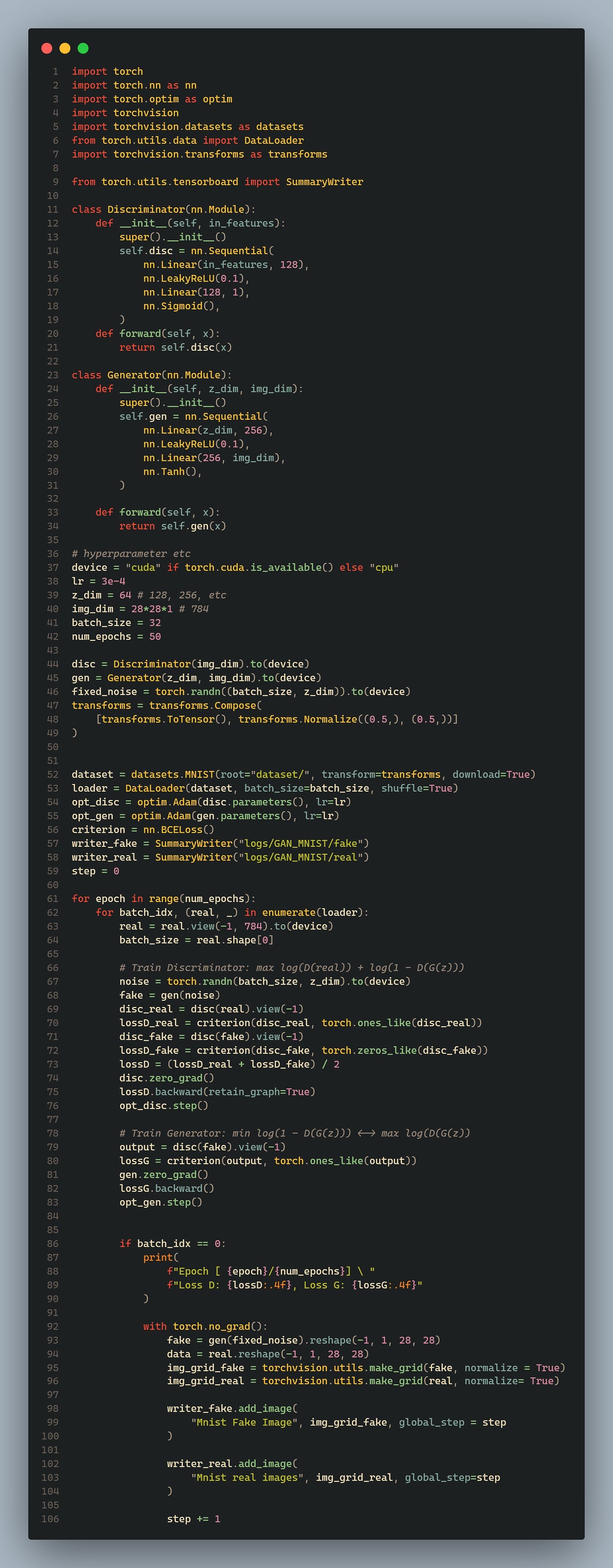
The above code is a very simple implementation of GAN, I will use this to expand on the concept talked about in part 1.
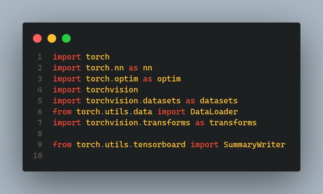
These lines import the necessary libraries for implementing a Generative Adversarial Network (GAN) using PyTorch. This includes modules for defining neural network architectures (torch.nn), optimization algorithms (torch.optim), datasets (torchvision.datasets), data loaders (torch.utils.data.DataLoader), image transformations (torchvision.transforms), and TensorBoard for visualization (torch.utils.tensorboard.SummaryWriter).
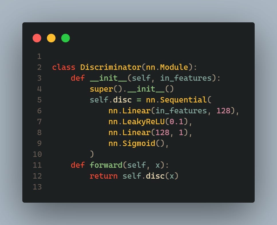
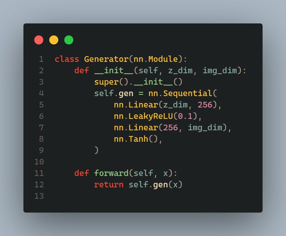
These classes define the architecture of the discriminator and generator neural networks, respectively. The discriminator takes an input of size in_features and outputs a single value indicating the probability that the input is real. The generator takes a random noise vector of size z_dim and outputs an image of size img_dim.
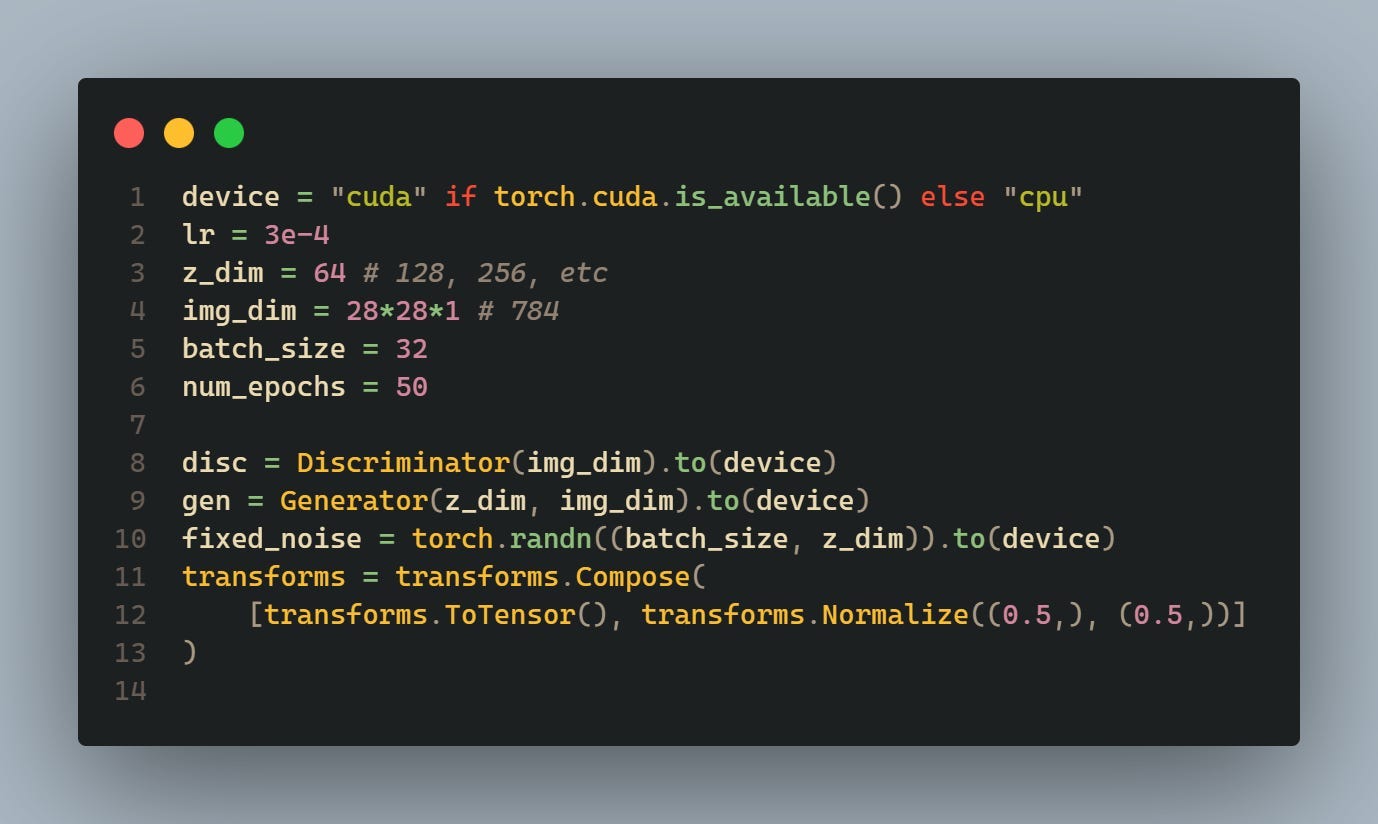
These lines set hyperparameters such as learning rate (lr), latent space dimension (z_dim), image dimension (img_dim), batch size (batch_size), and number of epochs (num_epochs). The device is set to GPU (“cuda”) if available, otherwise to CPU.
Also, instances of the discriminator and generator classes are created and moved to the specified device (CPU or GPU). fixed_noise is a fixed random noise vector used for generating fake images during training.
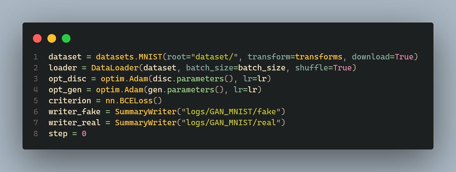
The MNIST dataset is then loaded using these transformations into a DataLoader, which will provide batches of data during training.
The Adam optimizers are defined for both the discriminator (opt_disc) and the generator (opt_gen). The learning rate (lr) is specified for both optimizers. Additionally, the Binary Cross Entropy (BCE) loss function (criterion) is defined, which will be used to calculate the loss during training.
Two SummaryWriter objects are created for logging fake and real images during training. These will be used to visualize the generated and real images using TensorBoard.
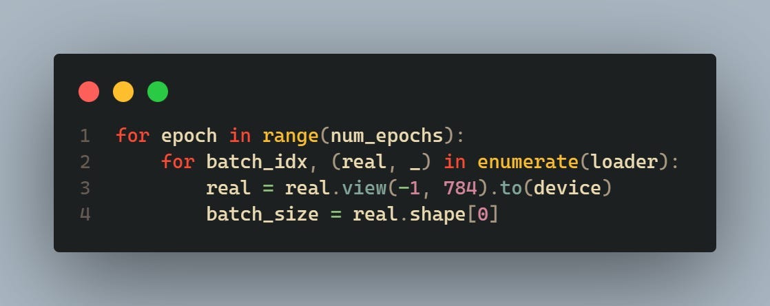
This loop iterates over each epoch and each batch of the dataset. It extracts real images (real) and their labels from the DataLoader. The real images are reshaped to a vector format (view (-1, 784)) and moved to the specified device (device).
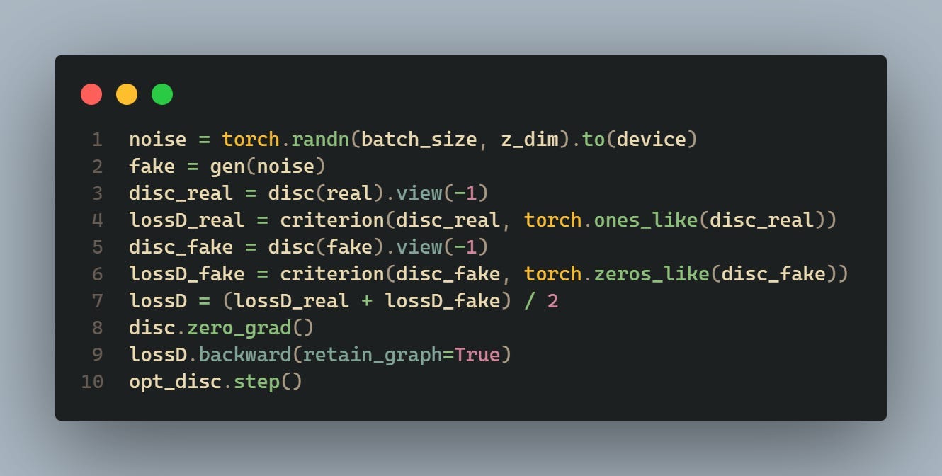
This part of the code trains the discriminator. First, random noise (noise) is generated and passed through the generator to produce fake images (fake). The discriminator evaluates both real and fake images and calculates the losses (lossD_real and lossD_fake) using the BCE loss function. Then, the total discriminator loss (lossD) is calculated as the average of the losses on real and fake images. Gradients are cleared (disc.zero_grad()), and backpropagation is performed (lossD.backward()), followed by an optimization step (opt_disc.step()).
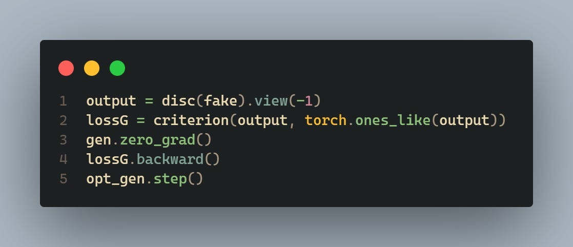
This section trains the generator. It evaluates the fake images produced by the generator using the discriminator and calculates the generator loss (lossG) based on the discriminator’s output. Gradients of the generator are cleared (gen.zero_grad()), backpropagation is performed (lossG.backward()), and an optimization step is taken (opt_gen.step()).
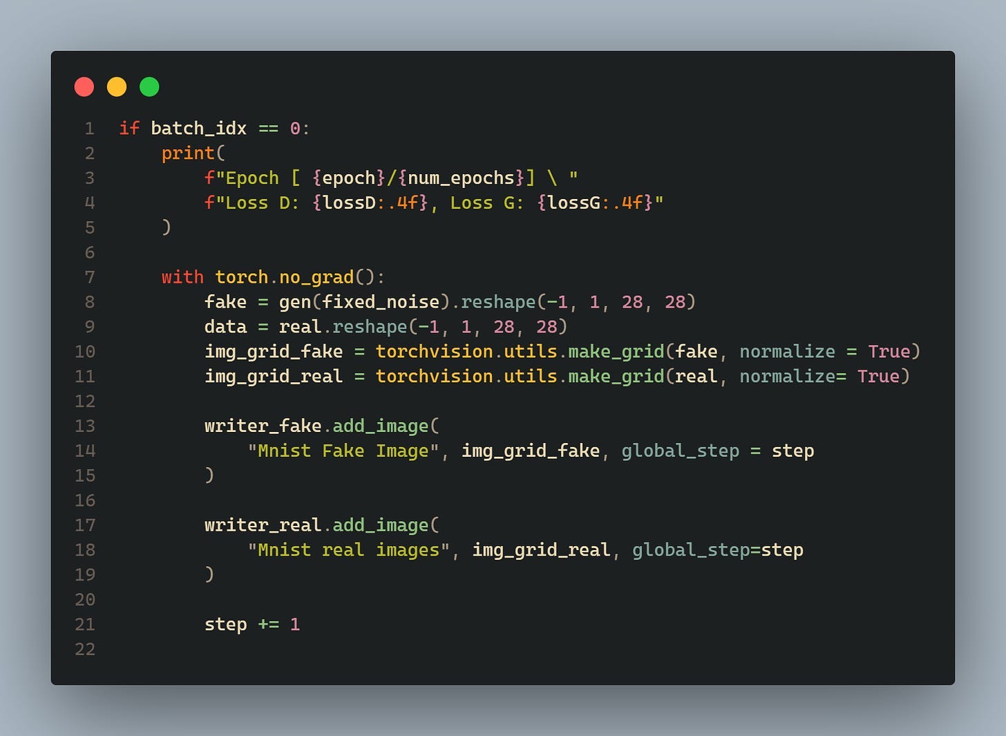
This part of the code is executed at the beginning of each epoch (when batch_idx == 0). It generates fake images using the generator (fake), creates image grids for fake and real images, and adds them to TensorBoard for visualization.
Thanks for reading this article, if you are interested in more things like this, you can subscribe to my substack here.