Introduction
Gradient Descent (GD) is a first order optimization algorithms that is used to find the minimum of a given function, it is commonly used in training machine learning and deep learning algorithms.
In machine learning after you train a model you would like to check how the model performed either by checking the accuracy or any other measure that suites the problem, let’s say you generate a **cost function **which is a measure of how wrong the model is finding a relationship between the input and the output, this is where Gradient Descent comes in, the gradient descent algorithm will optimize the cost function, it will give the minimum value of possible error of your model.
Gradient descent works for functions that are differentiable and convex.
Firstly, from calculus, derivative of a function is:

or some may know it as:

Secondly, A convex function is a continuous function whose value at the midpoint of every interval in its domain does not exceed the arithmetic mean of its values at the ends of the interval, or easier said, a convex function is like a bowl, curving upwards. This means that any line segment connecting two points on the curve lies above the curve itself. In other words, if you pick two points on a convex curve and draw a straight line between them, the curve will always be below or touching that line.
Mathematically:
A function f(x) is convex if, for any two points x1 and x2 in its domain and any λ in the interval [0,1], the following inequality holds:

This inequality essentially states that the function lies below the straight line connecting the two points (x1, f(x1)) and (x2, f(x2)) for any choice of λ between 0 and 1. If this condition holds for all pairs of points and all λ, then the function is convex. You can learn more here
a simpler way to know whether it is convex is to check whether the second derivative of the function is greater than 0.

The Gradient Descent algorithm
The whole idea of the gradient algorithm is to calculate the next point to converge using the gradient of the function at the current position, this is then multiplied by the learning rate and then subtracts obtained value from the current position, the reason is simply to minimize the function, maximizing will be adding.
Learning rate is a parameter in gradient descent algorithm also referred to as step size is the size of the steps that are taken to reach the minimum. It is typically a small value, and it is evaluated and updated based on the behavior of the cost function. High learning rate may result to overshooting or diverging completely, conversely low learning rate can result to more time to reach the minimum.

In this formula:
θi+1 represents the updated parameter values in the next iteration.
θi represents the current parameter values.
α is the learning rate, a positive scalar that determines the step size.
∇J(θi) represents the gradient of the cost (or loss) function J with respect to the parameters θi.
The formula represents how the parameters are updated in each iteration of the gradient descent algorithm to minimize the cost function.
Implementation
GD implementation steps are:
Initialization: choose a starting point on the function
Gradient: calculate the gradient at that point
Descend: make a step to the new position using the gradient descent formula
Repeat: the process goes on until the minimum of the function or the maximum number of iterations is reached.
Let’s say we have a function:

the derivative becomes:

In python:
Then we have our gradient descent implementation:
calling the function:

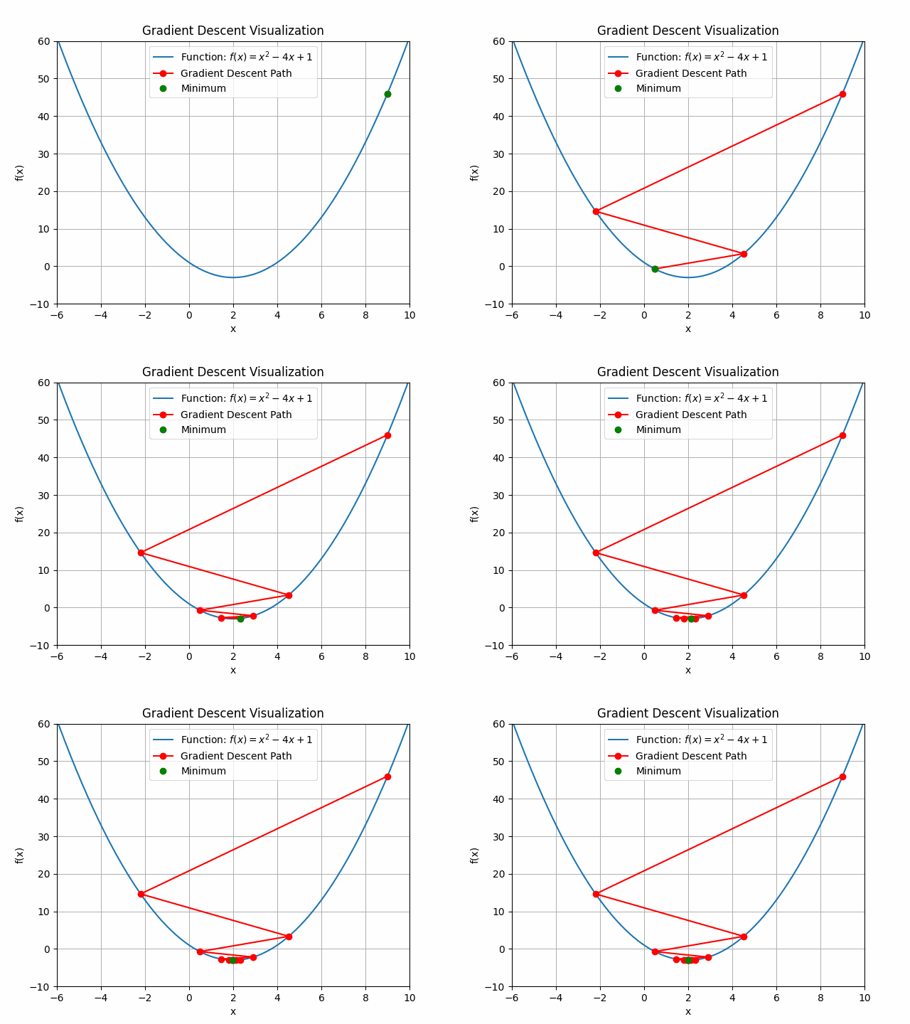
The animation above shows how to Gradient descent algorithm when the learning rate is 0.01, when the learning rate is increased to something like 0.9.

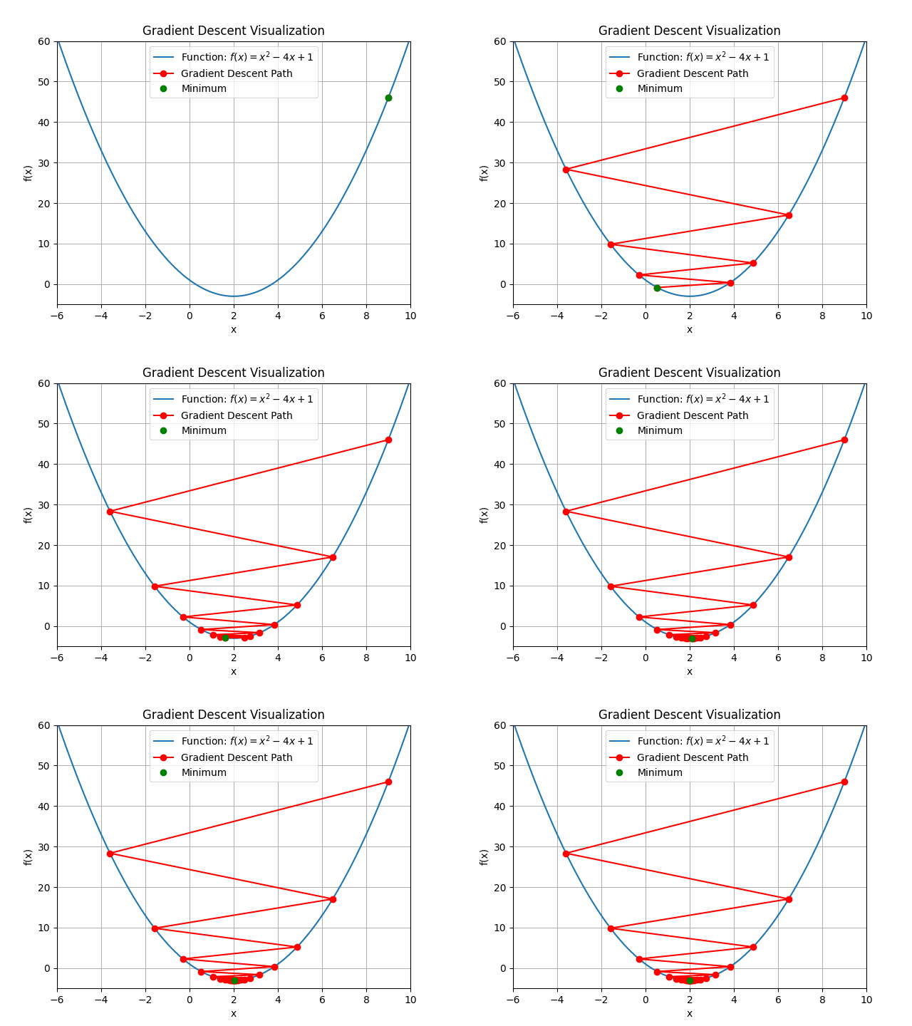
Let’s check out learning rate 1.0!

You can see that for bigger learning rate it starts to jump from side to side, so as we increase the learning rate it may eventually diverge.
Challenges with Gradient Descent
Vanishing Gradient: This mostly occurs when the gradient is too small, mostly in neural networks, during backpropagation, the gradient becomes smaller (vanishes) this causes the earlier layers of the network to learn slowly as this happens the weight update of the later part of the network become insignificant. You can check out more here or here
Exploding Gradient: This is more like the inverse of vanishing gradient problem, here the gradient is too large, and it creates a very unstable model you can check out more here
You can get the code for the visualization here
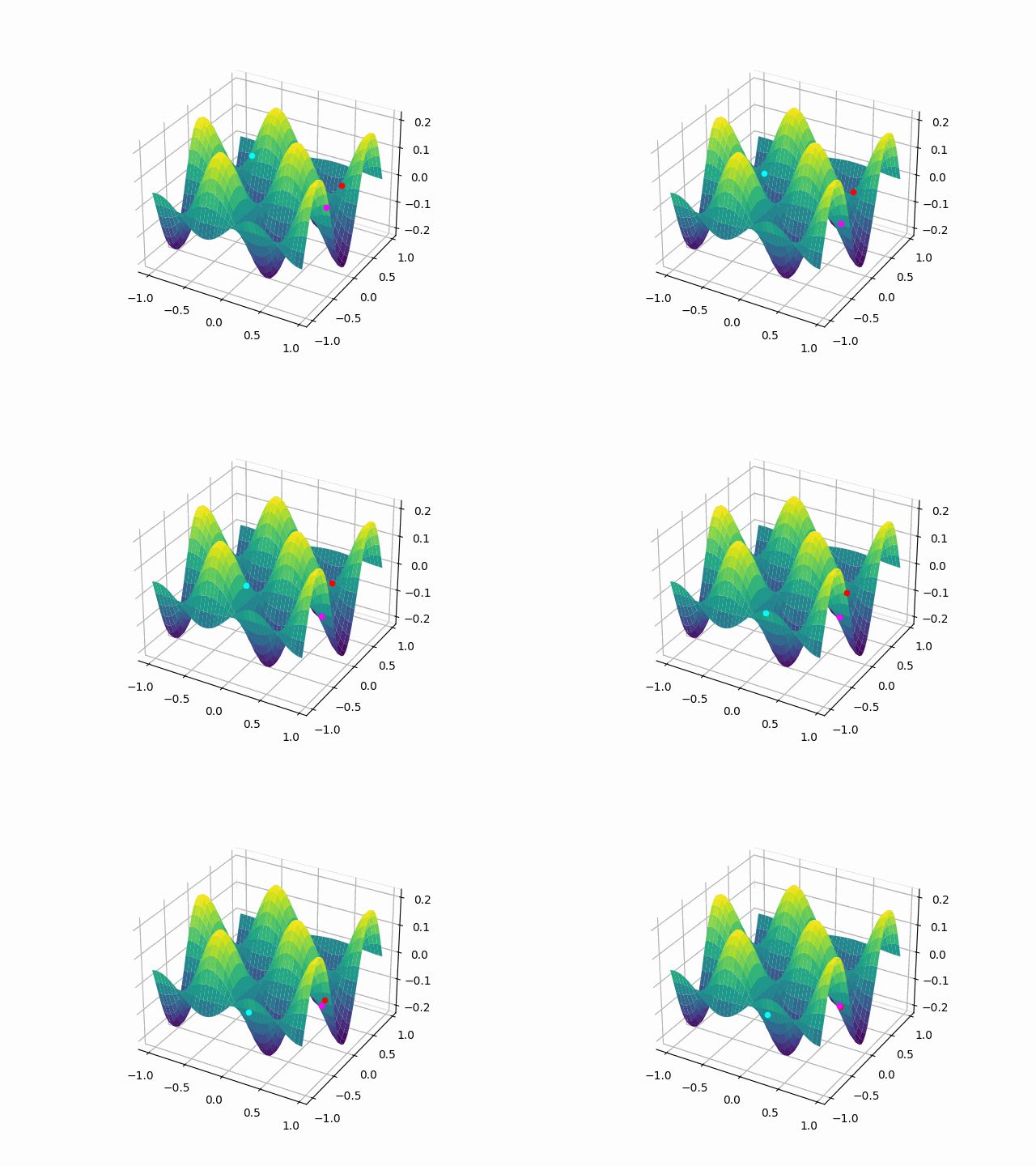
If you made it to the end, here is a cool visualization for you :)
