In our daily lives, we encounter the concept of distance in various forms and contexts. Whether we’re navigating through a busy city, exploring the vastness of the universe, or even contemplating the emotional space between ourselves and others, distance plays a fundamental role in shaping our experiences and understanding of the world. But did you know that distance can be perceived and measured in numerous ways, each offering unique insights into the relationships between objects, ideas, and individuals?
I am going explain and give the code from easy to hard on my preferences 🙂
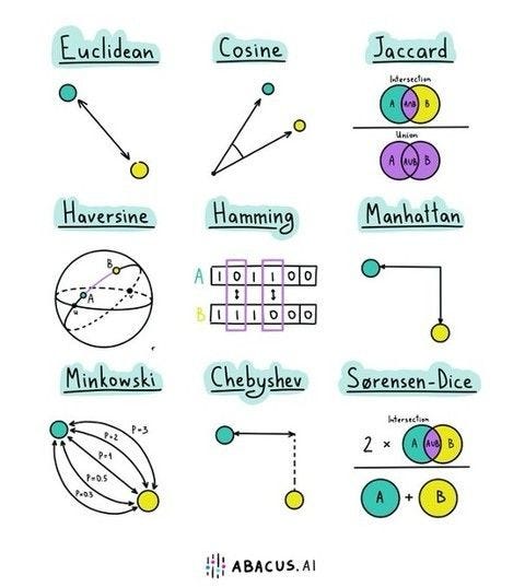
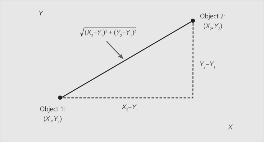
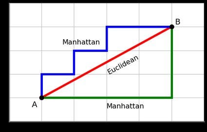
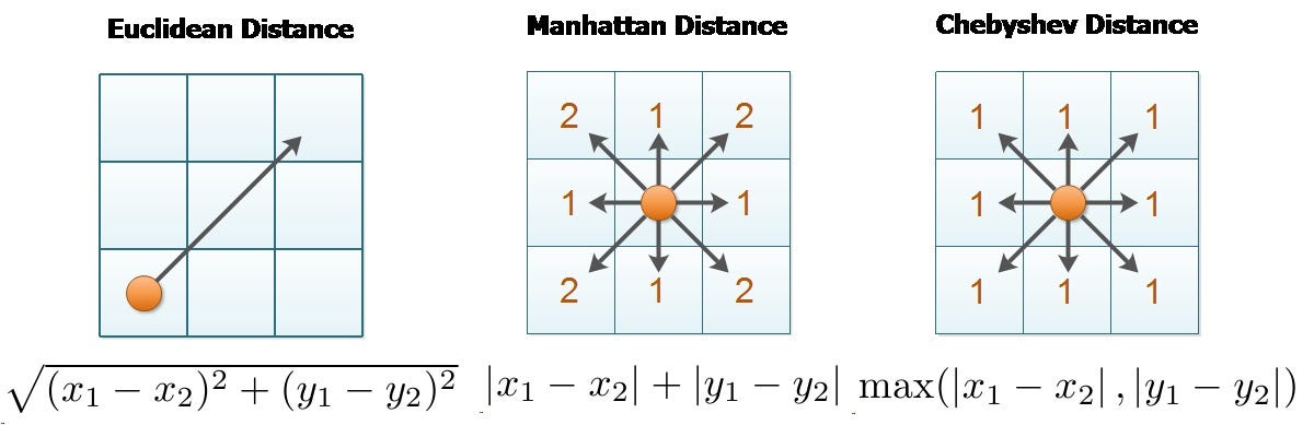
Euclidean Distance: Euclidean distance is a widely used distance metric that measures the straight-line distance between two points in a multidimensional space. In a 2D space, Euclidean distance represents the length of the straight line connecting two points on a Cartesian plane. In 3D space, it measures the distance between two points in a three-dimensional coordinate system. The formula for Euclidean distance is derived from the Pythagorean theorem.
    import numpy as np

    def euclidean_distance(point1, point2):
        """Calculate the Euclidean distance between two points."""
        return np.sqrt(np.sum((point1 - point2) ** 2))
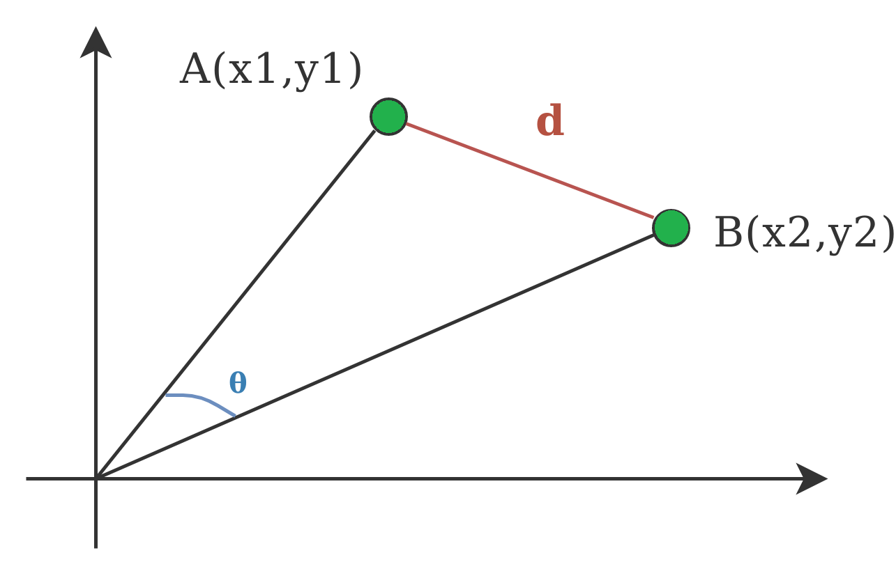
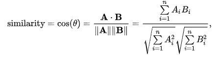
Cosine Distance: Cosine distance is a similarity metric used to quantify the angle between two vectors in a high-dimensional space. It measures the cosine of the angle between the vectors, representing how similar or dissimilar they are. it excels in sparse data, magnitude intensive, textual data, implicit feedback (recommender systems). 1- cosine similarity is cosine distance.
    import numpy as np

    def cosine_distance(point1, point2):
        """Calculate the cosine distance between two points."""
        return 1 - np.dot(point1, point2) / (np.sqrt(np.dot(point1, point1)) * np.sqrt(np.dot(point2, point2)))
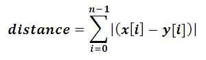
Manhattan Distance: Manhattan distance is a distance metric that calculates the distance between two points in a grid-like, rectilinear space. Mathematically, Manhattan distance is the sum of the absolute differences between the coordinates of two points. compared to Manhattan distance, Euclidean distance calculates the straight-line distance between two points, considering both horizontal and vertical movements, while Manhattan distance measures the distance in a grid-like space, considering only horizontal and vertical movements. Manhattan distance is less sensitive to high-dimensional data, as it sums absolute differences instead of squaring them like Euclidean distance. Additionally, Manhattan distance is more interpretable, representing the total blocks one must walk in a grid-like space to reach the destination. The choice between the two metrics involves trade-offs; Euclidean distance treats all directions equally, making it suitable for cases with diagonal movements, while Manhattan distance is computationally efficient and better suited for scenarios with grid-like movements or high-dimensional data.
    import numpy as np

    def manhattan_distance(point1, point2):
        """Calculate the Manhattan distance between two points."""
        return np.sum(np.abs(point1 - point2))
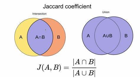
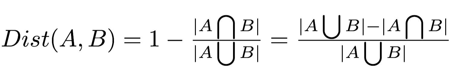
Jaccard similarity: Jaccard distance is a distance metric that quantifies the dissimilarity between two sets based on their elements’ uniqueness. It is calculated as 1 minus the Jaccard similarity, which is the size of the intersection of the sets divided by the size of their union. Jaccard distance is directly related to set similarity, as it measures how much the sets differ from being identical. This distance metric finds extensive applications in analyzing data with categorical features or binary data, where the presence or absence of items matters more than their actual values. For instance, it is used in text mining for document similarity, where documents are represented as sets of words. In recommendation systems, Jaccard distance helps identify similar users or items based on their shared preferences or characteristics. It is more appropriate than other metrics when dealing with data that can be efficiently represented as sets, especially when the data lacks a continuous nature.
    def jaccard_distance(set1, set2):
        intersection = len(set1.intersection(set2))
        union = len(set1.union(set2))
        return 1 - (intersection / union)
Haversine distance: Haversine distance is a formula used to calculate the shortest distance between two points on the Earth’s surface, assuming the Earth is a perfect sphere. It is specifically designed for measuring great-circle distances, making it suitable for geographical applications and GPS systems. Unlike other distance metrics, Haversine distance accounts for the Earth’s curvature, making it more accurate for long distances and near the poles. It overcomes challenges posed by simple Euclidean distance calculations on flat surfaces, which can lead to significant errors when applied to the Earth’s curved surface. Therefore, Haversine distance is a crucial tool for accurately estimating distances in geographic calculations and navigation systems that involve long-distance travel.
    from math import radians, sin, cos, sqrt, atan2

    def haversine_distance(lat1, lon1, lat2, lon2):
        """Calculate the haversine distance given latitude and longitude"""
        R = 6371.0  # Earth radius in kilometers

        lat1, lon1, lat2, lon2 = map(radians, [lat1, lon1, lat2, lon2])

        dlat = lat2 - lat1
        dlon = lon2 - lon1

        a = sin(dlat / 2)**2 + cos(lat1) * cos(lat2) * sin(dlon / 2)**2
        c = 2 * atan2(sqrt(a), sqrt(1 - a))

        return R * c
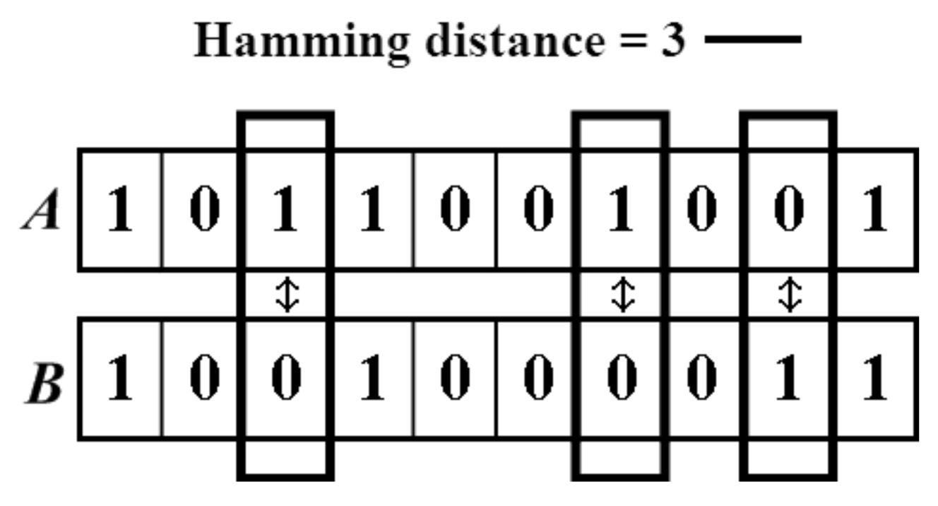
Hamming Distance: Hamming distance is a metric used to measure the dissimilarity between two strings of equal length by counting the number of positions at which the corresponding characters differ. Its simplicity and efficiency make it a valuable tool in various domains where binary data is prevalent, including telecommunications, DNA sequence analysis, and error-tolerant matching algorithms. For example, in the picture below counting from left, the dissimilarities on the two binary codes occured 3 times.
    def hamming_distance(str1, str2):
        return sum(c1 != c2 for c1, c2 in zip(str1, str2))
**Minkowski Distance: **Minkowski distance is a distance metric that generalizes both Euclidean and Manhattan distances. It measures the distance between two points in a multidimensional space using the formula below:

where 𝑥𝑖 and 𝑦𝑖 are the coordinates of the two points, and 𝑝 is a parameter that determines the distance’s behavior. When 𝑝=2, it becomes the Euclidean distance, and when 𝑝=1, it becomes the Manhattan distance. The value of 𝑝 governs the “order” of the Minkowski distance. For 𝑝>1, the distance emphasizes larger differences between coordinates, making it sensitive to outliers. For 𝑝<1, it emphasizes smaller differences, making it robust to outliers. Thus, Minkowski distance can adapt to different data distributions by adjusting the value of 𝑝, allowing for various distance behaviors that suit specific data characteristics and analysis requirements.
    import numpy as np

    def minkowski_distance(x, y, p):
        return np.sum(np.abs(x - y) ** p) ** (1 / p)
Chebyshev Distance: Chebyshev distance, also called L∞ norm, is a distance metric that measures the maximum difference along any dimension between two points. Imagine walking on a chessboard, where you can move horizontally, vertically, or diagonally by one step. The Chebyshev distance tells us the maximum number of steps we need to reach the destination. It’s helpful in scenarios like finding the shortest path on a chessboard or detecting outliers in data, where we want to identify extreme values that are farthest from the rest. So, Chebyshev distance helps us find the biggest difference and is useful in games, analyzing grids, and spotting unusual things in data.
In chess, all the three distances are used as follows; the distance between squares on the chessboard for rooks is measured in **Manhattan distance. **Kings and queens use **Chebyshev distance. **Bishops use the Manhattan distance (between squares of the same color) on the chessboard rotated 45 degrees, i.e., with its diagonals as coordinate axes. To reach from one square to another, only kings require the number of moves equal to the distance (Euclidean distance) rooks, queens and bishops require one or two moves. (source)
    import numpy as np

    def chebyshev_distance(x, y):
        return np.max(np.abs(x - y))
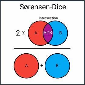
Sørensen-Dice Distance: Sorensen distance, also known as Sørensen–Dice coefficient, is a similarity measure between sets. It calculates the dissimilarity between two sets based on the proportion of common elements relative to the total elements in both sets. It is particularly useful in image segmentation and clustering tasks, where it helps identify similarities between regions or objects in images.
Imagine you have two sets of toys. The Sorensen distance, or Sørensen–Dice coefficient, helps you find out how much the two sets are alike. It counts how many toys are the same in both sets and then divides that number by the total number of toys in both sets. The result shows how similar or different the two sets are.
The difference between Sorensen distance and Jaccard similarity is how they measure similarity. Both use the number of shared toys between sets, but Sorensen distance also considers the total number of toys in each set, whereas Jaccard similarity only looks at the shared toys’ proportion. So, they are similar but have a slight difference in how they measure similarity between sets.
    def sorensen_distance(set1, set2):
        intersection = len(set1.intersection(set2))
        return 1 - (2 * intersection) / (len(set1) + len(set2))